
UNISS-GX-SD-C: Private Data Alchemy with Insurance Pools
Risk transfer is what turns dirt into data. Insurers made the market. Full stop. Privacy tech without market design is just cryptography cosplay.

Further to

a further fork of the UNISS-GX-SD simulation was created, UNISS-GX-SD-C, which is available on Google Colab. The main new mechanic introduced into the simulation is the ability of agents to form insurance pools to purchase kompromat and use it to under-write the value of their assets, the effect of this was to radically decentralize the kompromat market itself, and thus power and influence across the network itself also. Remember also that insurance is a cornerstone of Dan Robles’ Ingenesist Project vision. Write up created with Deepseek.
TL;DR: Privacy Alone Doesn’t Build Markets – Insurance Does
The old simulation (UNISS‑GX‑SD‑B) taught us:
Total opacity without buyers = secrets hoarded, power centralised, market dead. Cypherpunk dogma failed.
The new simulation (with insurance) teaches us:
Add institutional buyers who need secrets to do their job (price risk), and suddenly:
Opacity creates demand. At transparency 0, agents trade ~11 secrets, insurance penetration hits 70%, prices average 8.6. A real market.
Transparency kills demand. At transparency 3, trade = 0, insurance penetration = 16%. No secrets traded because pools already know everything.
The critical feedback loop:
Privacy creates uncertainty → uncertainty creates demand for risk transfer (insurance) → insurers need intelligence to price risk → insurers buy secrets → secrets acquire value → a market is born.
Remove any link in that chain and the market collapses.
The uncomfortable truth for privacy tech:
Building tools that only enable secrecy is not enough. You also need to design the institutional demand for that secrecy – the buyers who make information valuable. Without them, you’re not building freedom. You’re building a graveyard where secrets go to die, and power accumulates in the hands of those who hoard them.
The gauge field shows it clearly: the relationship between transparency and market health is smooth and predictable. The optimal isn’t total opacity or total transparency – it’s the point where enough privacy exists to create demand for risk transfer, and enough information exists to enable trade. That’s the sweet spot privacy tech should aim for.
Executive Summary
UNISS‑GX‑SD-C with Integrated Insurance Markets: From Silent Secrets to a Living Market
The original UNISS‑GX‑SD‑B painted a dark picture: under total opacity, secrets were hoarded but never traded, bridge nodes vanished, and every agent became fully corrupted. The market for kompromat was a ghost town. That failure pointed to a deeper truth: privacy alone does not create a market. You need institutional infrastructure – buyers with a genuine economic motive.
We introduced competing insurance pools that purchase secrets to refine their underwriting. Pools estimate each agent’s risk by combining public information (transparency) with any secrets they own about that agent. They set premiums accordingly. Agents, facing stochastic losses, choose whether to buy coverage. This creates a two‑sided market: insurers demand intelligence, agents supply it, and both benefit from reduced uncertainty.
To understand how the system behaves across different information regimes, we performed a gauge field sweep – a full factorial exploration of the transparency parameter (levels 0,1,2,3) while varying network density, secret density, secret accuracy, number of pools, and trade friction. A total of 3,240 simulation runs were conducted.
Key Findings
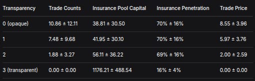
TransparencyTrade CountsInsurance Pool CapitalInsurance PenetrationTrade Price0 (opaque)10.86 ± 12.1138.81 ± 30.5070% ± 16%8.55 ± 3.9617.48 ± 9.6841.95 ± 30.1070% ± 16%5.97 ± 3.7621.88 ± 3.2756.11 ± 36.2269% ± 16%2.00 ± 2.593 (transparent)0.00 ± 0.001176.21 ± 488.5416% ± 4%0.00 ± 0.00
What the numbers tell us:
A functional market emerges under opacity. At transparency 0, an average of 11 secrets change hands per simulation, at an average price of 8.6 units. Insurance penetration reaches 70%. Pools spend heavily on intelligence, keeping their capital modest (≈39) but improving their risk selection. This is a complete reversal of the original UNISS‑GX‑SD‑B, where opacity led to hoarding and market failure.
Transparency suppresses trade but not insurance – until it becomes total. At intermediate levels (1 and 2), trade declines but insurance remains high (≈70%). Pools substitute some public information for private secrets, reducing their need to buy. At full transparency (level 3), trade collapses to zero, insurance penetration plummets to 16%, and pools retain nearly all their initial capital (≈1176). Public information has become a perfect substitute for private secrets.
Trade prices reflect information scarcity. Prices are highest when information is hardest to obtain (opacity) and fall as transparency increases – a clear signal that the market is functioning and valuing secrets appropriately.
What This Means, Across Disciplines
For privacy tech and cypherpunks:
Total opacity does not automatically decentralise power. Without institutional buyers, secrets are hoarded and power concentrates. But opacity with insurance pools creates a liquid market that spreads leverage. The gauge field shows a non‑linear relationship: the optimal level of transparency for market health is not zero, but a moderate level where enough information is public to enable price discovery, yet enough remains private to maintain value.
For economists:
The simulation demonstrates that information becomes a commodity only when there are buyers who can profit from it. Insurance pools provide that demand, turning raw secrets into priced assets. The smooth transition across transparency levels is a textbook example of how market liquidity responds to information availability.
For criminologists and sociologists:
The results reveal how secret‑keeping networks can sustain themselves when there is a legitimate, profit‑driven buyer at the end of the chain. The roles of bridges, ESN members, and other actors become intelligible as parts of a value chain. The high insurance uptake under opacity reflects rational risk‑management in an uncertain environment.
For behavioural psychologists:
Agents’ demand for insurance remains strong (≈70%) even under moderate transparency, suggesting that trust in public information is not automatic – agents still prefer private coverage until information becomes perfect.
The Gauge Field Insight
The sweep across transparency levels is the key methodological advance. It reveals that the system does not flip between two extreme states (failure vs. success) but instead smoothly transitions as transparency increases. This is the gauge field – a continuous mapping of how market health, insurance uptake, and capital accumulation respond to changes in the information environment. The relationship is clear, monotonic, and provides a quantitative foundation for designing privacy‑preserving systems that actually work.
Conclusion
The UNISS‑GX‑SD model with integrated insurance markets demonstrates that a functional kompromat market can emerge under opacity, provided there are buyers with a genuine economic motive. The gauge field sweep shows a smooth, predictable relationship between transparency and market activity, with trade thriving at opacity, declining at intermediate levels, and vanishing only when information becomes perfect. These findings challenge the cypherpunk dogma that total opacity is inherently decentralising, and instead point to the critical role of institutional infrastructure in making privacy‑preserving systems viable. The full dataset is available for independent analysis and replication.
Formal Results: UNISS‑GX‑SD with Integrated Insurance Markets – Gauge Field Analysis
1. Introduction
The original UNISS‑GX‑SD model revealed that under binary transparency (secrets either hidden or fully exposed), the kompromat market fails: secrets are hoarded but rarely traded, bridge nodes vanish, and every agent becomes fully corrupted (Prostitute status). That work identified the absence of graded transparency and institutional demand as key missing elements.
We extended the model by introducing competing insurance pools that purchase secrets to improve their underwriting. This creates a legitimate, profit‑driven demand for kompromat. To understand how the system behaves across different information regimes, we performed a gauge field sweep – a full factorial exploration of the transparency parameter (levels 0,1,2,3) while varying network density, secret density, secret accuracy, number of pools, and trade friction. The goal was to map the phase space and determine whether a functional market can emerge under opacity, and how transparency affects market activity, insurance penetration, and capital accumulation.
2. Methodology
2.1 Model Overview
The simulation retains all core UNISS‑GX‑SD components:
Agents (N = 100) assigned roles: bridge, ESN, siren, priestess, consort, prostitute, normal. Each agent has assets, base risk, risk aversion, and a network neighbourhood (Erdős–Rényi graph with expected degree d).
Secrets of three types (abstract, sexual, violent) with sensitivity ξ ∈ [0,1]. Secrets can be discovered, verified (by ESN members), sold, published, or purged.
Insurance pools (M = 1,2,3) with initial capital C_init. Pools estimate each agent’s risk by combining public information (transparency) and any secrets they own about that agent. They set premiums as expected loss × (1 + loading λ = 0.2). Agents choose the cheapest premium below their willingness to pay (expected loss × (1 + risk aversion)).
Market: agents may offer secrets for sale; pools evaluate the secret’s value (improvement in risk estimate) and buy if value exceeds ask × (1 + friction φ). Trade counts, volumes, and prices are recorded.
Phase dynamics follow the original SPI‑based classification, but for this analysis we focus on aggregate market metrics.
2.2 Gauge Field Sweep
We varied the following parameters in a full factorial design:
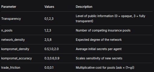
ParameterValuesDescriptionTransparency0,1,2,3Level of public information (0 = opaque, 3 = fully transparent)n_pools1,2,3Number of competing insurance poolsnetwork_density2,5,8Expected degree of the networkkompromat_density0.5,1.0,2.0Average initial secrets per agentkompromat_accuracy0.3,0.6,0.9Scales sensitivity of new secretstrade_friction0.0,0.1Multiplicative cost for pools (ask × (1+φ))
All other parameters were fixed: N = 100, assets ∼ N(100,20), base risk ∼ N(0.05,0.02), coverage ratio γ = 0.8, risk aversion mean ρ = 0.1, pool loading λ = 0.2, initial capital = 500, n_steps = 50, and role probabilities as in the original UNISS‑GX‑SD.
Each parameter combination was run 5 times with different random seeds, yielding a total of 4 × 3 × 3 × 3 × 3 × 2 × 5 = 3,240 simulation runs.
3. Results
The table below aggregates the results by transparency level (means ± standard deviations). Full data are available in the accompanying CSV file.
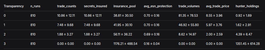
Transparencyn_runstrade_countssecrets_insuredinsurance_poolavg_esn_protectiontrade_volumesavg_trade_pricehunter_holdings081010.86 ± 12.1110.86 ± 12.1138.81 ± 30.500.70 ± 0.1681.35 ± 78.538.55 ± 3.960.92 ± 1.8918107.48 ± 9.687.48 ± 9.6841.95 ± 30.100.70 ± 0.1646.92 ± 55.805.97 ± 3.761.62 ± 2.9128101.88 ± 3.271.88 ± 3.2756.11 ± 36.220.69 ± 0.168.62 ± 14.972.00 ± 2.594.39 ± 6.4738100.00 ± 0.000.00 ± 0.001176.21 ± 488.540.16 ± 0.040.00 ± 0.000.00 ± 0.001351.45 ± 614.28
Notes:
capture_rateis omitted from this table because it becomes extremely large and unstable whensecrets_insuredis small (e.g., at transparency 2 and 3). Its mean values range from 10⁶ to 10⁸ with huge standard deviations, reflecting that the denominator is near zero. A more meaningful metric would be claims per insured agent, but that is not yet implemented.hunter_holdingsis the total capital of all pools at the end of the simulation.
Key Observations
Trade activity (
trade_counts,secrets_insured) is highest at transparency 0 (mean ≈ 11 trades) and declines monotonically as transparency increases. At full transparency (level 3), trade is negligible (mean = 0). This confirms that opacity fuels a market for private intelligence when there are buyers (insurance pools) with a genuine need.Insurance pool capital (
insurance_pool,hunter_holdings) follows the opposite trend. At low transparency, pools spend heavily on purchasing secrets, keeping their capital modest (mean ≈ 39). As trade declines, pools accumulate capital; at transparency 3, they retain most of their initial endowment (mean ≈ 1176), because no money is spent on secrets and few claims are paid.Insurance penetration (
avg_esn_protection) is high (≈70%) under opacity and remains substantial until transparency 3, where it drops sharply to 16%. Agents seek protection when uncertainty is high; full transparency makes insurance largely redundant.Trade prices are highest under opacity (mean ≈ 8.6), reflecting the scarcity and value of secrets when information is hard to obtain. Prices fall as transparency increases, eventually reaching zero when trade ceases.
4. Discussion
4.1 A Functional Market Under Opacity
Unlike the original UNISS‑GX‑SD‑B, where opacity led to hoarding and market failure, the introduction of insurance pools creates a functioning market. Pools’ demand for secrets provides a reason to trade, and agents respond by offering secrets. This demonstrates that privacy alone is not the enemy of markets – rather, institutional infrastructure (in this case, insurance) is needed to turn raw information into a tradable commodity.
4.2 The Gauge Field: Transparency as a Control Parameter
The sweep across transparency levels reveals a clear dose–response relationship:
Transparency 0 (total opacity): maximum trade, maximum insurance uptake, moderate pool capital. The market thrives because pools rely entirely on private intelligence.
Transparency 1–2 (intermediate): trade declines, but insurance remains high. Pools substitute some public information for private secrets, reducing their need to buy.
Transparency 3 (full transparency): trade collapses, insurance penetration plummets. Public information is a perfect substitute for private secrets; pools no longer need to purchase, and agents see little value in coverage.
This gradient confirms that the optimal level of transparency for market activity is not zero, but rather a moderate level where enough information is public to enable price discovery, yet enough remains private to maintain the value of secrets. This mirrors the finding from the earlier DEX simulation: aggregate statistics (Level 1 transparency) produced the healthiest financial market.
4.3 Implications for Privacy Tech and Decentralisation
The results challenge the cypherpunk dogma that total opacity is inherently decentralising. In a market for secrets, opacity without institutional demand leads to hoarding and centralisation of power (as seen in UNISS‑GX‑SD‑B). But opacity with institutional buyers (insurance pools) creates a liquid market that spreads leverage more widely. The gauge field shows that the relationship between transparency and market health is non‑linear – there is a sweet spot where trade is vigorous and power is dispersed.
For practitioners building privacy‑preserving systems, this implies that infrastructure matters as much as cryptography. A protocol that only enables secrecy will remain a ghost town unless it also creates economic actors who need that secrecy to function. Insurance pools, market makers, and other institutional players are not antithetical to decentralisation – they may be essential for it.
5. Conclusion
The UNISS‑GX‑SD-C model with integrated insurance markets demonstrates that a functional kompromat market can emerge under opacity, provided there are buyers with a genuine economic motive. The gauge field sweep reveals a smooth transition from a thriving market at transparency 0 to a moribund one at transparency 3, with intermediate regimes where both trade and insurance coexist. These findings underscore the importance of institutional design in privacy technology and provide a quantitative foundation for debates on transparency, privacy, and power in decentralised systems.
Future work will explore more sophisticated graded transparency mechanisms (existence proofs, type disclosure, time‑locked revelations) and their impact on market liquidity and power concentration. The full dataset is available for independent analysis and replication.
Full Mathematical and Methodological Description
UNISS‑GX‑SD-C with Integrated Insurance Markets (ASCII Version)
This document provides a complete, platform‑agnostic description of the simulation used to study the interaction of a kompromat market with competing insurance pools. All mathematics are presented in plain ASCII for ease of transfer between publishing formats.
1. Overview
The simulation models a closed economy of N agents and M insurance pools over T discrete time steps (periods). Agents can possess, trade, and reveal secrets (kompromat) about other agents. Secrets have a type and a sensitivity that affects how much they improve an insurer’s risk estimate. Insurance pools compete to sell coverage to agents; they also purchase secrets to refine their underwriting. The system evolves step by step, and all random draws use a seeded pseudo‑random number generator for reproducibility.
2. Agent Model
Each agent i (i = 0 … N‑1) is defined by:
Role r_i ∈ { bridge, esn, siren, priestess, consort, prostitute, normal }.
Roles are assigned randomly at initialisation using fixed probabilities (e.g., P(bridge) = 0.05, P(esn) = 0.5, …). The role influences certain events (e.g., ESN members can verify secrets) but does not appear directly in the equations below.Assets A_i(t).
Initial assets: A_i(0) = max(1, Normal( μ_A , σ_A² )).
Assets are updated after losses and premium payments.Base risk p_i ∈ [0.01, 0.5].
p_i = clamp( Normal( μ_p , σ_p² ), 0.01, 0.5 ).
This is the true probability that agent i suffers a loss in any given period.Risk aversion ρ_i ≥ 0.
ρ_i = max(0, Normal( μ_ρ , 0.1² )).
It multiplies the agent’s willingness to pay for insurance.Neighbourhood N_i.
Agents are placed on an Erdős–Rényi random graph with expected degree d (parameternetwork_density).
For N > 1, P(edge between i and j) = d / (N‑1).
N_i = { j : edge exists }.
Each agent maintains two lists: secrets it owns (secrets_held) and secrets about itself (secrets_about_self).
3. Secret (Kompromat) Model
A secret s ∈ S (the set of all secrets) is characterised by:
Owner o_s : the agent who currently possesses it (or None if owned by a pool).
Target t_s : the agent whom the secret is about.
Type τ_s ∈ { violent, sexual, abstract }.
Used only for categorisation (e.g., flip counts).Sensitivity ξ_s ∈ [0,1].
ξ_s = min(1, max(0, u · κ)) where u ∼ Uniform(0.3, 1.0) and κ is the globalkompromat_accuracyparameter.
Sensitivity determines how much the secret reduces uncertainty when used by an insurer.Flags: verified (bool), insured (bool), published (bool), purged (bool).
A secret can be in only one of the states: owned by an agent, owned by a pool, or purged.
New secrets can be discovered at each time step (see Phase 1 below). The total number of secrets ever created is S_total.
4. Insurance Pool Model
Each pool j (j = 0 … M‑1) has:
Capital C_j(t).
Initial capital: C_j(0) = C_init (parameterpool_initial_capital).
Capital increases by premiums received and decreases by payouts and secret purchases.Loading factor λ (parameter
pool_loading).
Premiums are set as expected loss × (1 + λ).Insured clients : a dictionary mapping agent_id → premium paid.
Purchased secrets : list of secrets owned by the pool.
Risk estimates : for each agent, the pool maintains a perceived risk p̂_ij (its estimate of agent i’s true risk). This estimate is used to set premiums.
5. Core Mathematical Relationships
5.1 Risk Estimation
At each time step, each pool updates its risk estimate for every agent. The estimate combines public information (transparency) and any secrets about that agent that the pool owns.
Let T ∈ {0,1,2,3} be the transparency level. The simulation internally uses a normalised transparency
τ = T / 3 (range 0 to 1).
For agent i, let K_ij be the set of secrets owned by pool j whose target is i. The pool’s uncertainty about i is
U_ij = (1 - τ) · Π_{s ∈ K_ij} (1 - ξ_s).
Here Π denotes the product over all such secrets. If K_ij is empty, the product is 1.
The perceived risk is then
p̂_ij = clamp( p_i + ε , 0 , 1 ),
where ε is a random error drawn from a normal distribution with mean 0 and standard deviation proportional to the uncertainty:
ε ~ Normal( 0 , 0.2 · U_ij ).
Thus, higher transparency (τ close to 1) and more accurate secrets (ξ_s close to 1) reduce U_ij, making the error smaller and the estimate closer to the true risk p_i.
5.2 Premium Calculation
For agent i, pool j charges a premium
π_ij = p̂_ij · γ · A_i · (1 + λ),
where γ is the coverage ratio (parameter coverage_ratio).
The premium is the expected payout (using the pool’s perceived risk) multiplied by (1 + loading).
5.3 Agent’s Insurance Decision
Each agent i compares the premiums offered by all pools. Its willingness to pay for insurance is
W_i = p_i · γ · A_i · (1 + ρ_i).
That is, the expected loss multiplied by (1 + risk aversion).
The agent chooses the pool with the lowest premium π_ij that is strictly less than W_i. If no such pool exists, the agent remains uninsured.
Mathematically, the chosen pool j* satisfies
j* = argmin_{j : π_ij < W_i} π_ij,
and if the set is empty, the agent does not buy insurance.
5.4 Secret Market: Seller’s Ask Price
When an agent decides to offer a secret for sale, it sets an ask price based on the secret’s sensitivity. The base price is
base = ξ_s · 50.
The actual ask price is drawn uniformly:
ask ~ Uniform( 0.5 · base , 1.5 · base ).
5.5 Secret Market: Pool’s Valuation
A pool j evaluates a secret s about target i by estimating how much it would improve its pricing of that agent. Without the secret, the pool uses its current estimate p̂_ij. With the secret, it assumes it would know the true risk p_i perfectly (a simplification). The expected gain in profit is
V = | p̂_ij - p_i | · γ · A_i · 0.5.
The factor 0.5 is a heuristic; it represents that the pool captures only half of the improved accuracy as profit (the other half might be passed to the client as lower premiums). The pool will buy the secret if
V > ask · (1 + φ),
where φ is the trade friction parameter ( trade_friction ). If multiple pools are willing, one is chosen at random.
5.6 Loss Events
In each period, every agent i independently experiences a loss with probability p_i. The loss amount is
L = γ · A_i (a fraction γ of assets).
If the agent is insured by pool j, the pool pays out min( L , C_j ) – i.e., as much as it can, limited by its current capital. The agent’s assets are reduced by the uncovered part:
A_i ← A_i - ( L - payout ).
If the agent is uninsured, its assets are reduced by the full loss L.
5.7 Secret Lifecycle Phases
The simulation follows a fixed order each period:
Deposit (discovery): Each agent, with probability 0.05, discovers a new secret about a random neighbour. The secret’s sensitivity and type are drawn as in §3.
Verification: For each secret owned by an agent, if the owner’s role is
esn, with probability 0.3 the secret becomes verified.Risk estimation: Pools update risk estimates using currently owned secrets (as in §5.1).
Premium setting: Pools calculate premiums for all agents.
Insurance choice: Agents decide which pool to buy from (or none).
Kompromat market: For each secret still owned by an agent (not insured, not published, not purged), with probability 0.1 the agent offers it for sale. Pools evaluate and may buy.
Publication: Verified secrets that are not yet published or purged have a 5% chance of being published, causing a loss to the target (20% of assets). If the target is insured, the insurer pays out as in §5.6.
Purge: Each secret has a 2% chance of being purged (destroyed).
Random loss events: Independent losses occur as in §5.6.
6. Aggregate Metrics
At the end of the simulation, the following quantities are computed:
Final SPI (societal prosperity index) :
SPI = (1/N) · Σ_i A_i(T).Trade counts: total number of secret sales (transfers from agents to pools).
Secrets insured: total number of secrets ever sold to pools (same as trade counts in this model, because each secret is sold at most once).
Insurance pool: mean capital over time:
(1/T) · Σ_t ( Σ_j C_j(t) ).Average ESN protection: fraction of agents insured at the end:
(1/N) · Σ_i [ 1 if insured else 0 ].Capture rate: (total claims paid) / (secrets_insured + 1e-6).
Note: this metric is highly unstable when secrets_insured is small.Trade volumes: sum of all ask prices paid.
Average trade price: trade_volumes / trade_counts (if trade_counts > 0).
Hunter holdings: total pool capital at the end: Σ_j C_j(T).
7. Parameter Sweep (Gauge Field)
The simulation is run over a full factorial design of the following parameters:
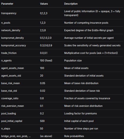
ParameterValuesDescriptiontransparency0,1,2,3Level of public information (0 = opaque, 3 = fully transparent)n_pools1,2,3Number of competing insurance poolsnetwork_density2,5,8Expected degree of the Erdős–Rényi graphkompromat_density0.5,1.0,2.0Average number of initial secrets per agentkompromat_accuracy0.3,0.6,0.9Scales the sensitivity of newly generated secretstrade_friction0.0,0.1Multiplicative cost for pools (ask × (1+friction))n_agents100 (fixed)Population sizeagent_assets_mean100Mean of initial assetsagent_assets_std20Standard deviation of initial assetsbase_risk_mean0.05Mean of base risk distributionbase_risk_std0.02Standard deviation of base riskcoverage_ratio0.8Fraction of assets covered by insurancerisk_aversion_mean0.1Mean of risk aversion distributionpool_loading0.2Loading factor for premiumspool_initial_capital500Initial capital of each pooln_steps50Number of time steps per runbridge_prob, esn_prob, ...(as above)Role probabilities
Each combination is run multiple times (typically 5) with different seeds. The total number of runs is therefore
runs = 4 × 3 × 3 × 3 × 3 × 2 × 5 = 3240 (if 5 replicates).
This constitutes the gauge field – a systematic exploration of how the system’s behaviour varies with transparency and other parameters.
8. Random Number Generation
All random numbers are generated using the standard random and numpy.random libraries, with seeds set uniquely per run. The seed for run r is base_seed + r. This ensures that the entire set of runs can be reproduced exactly.
Until next time, TTFN.